void mat_mul(float a[2][2], float b[2][3], float c[2][3]) {
    for (r = 0; r < 2; r++) {
        for (c = 0; c < 3; c++) {
            c[r][c] = 0;
            for (k = 0; k < 2; k++) {
                c[r][c] += a[r][k] * b[k][c];
            }
        }
    }
}15 May 2021
I recently read Vectorization for Digital Signal Processors via Equality Saturation by Alexa VanHuttum, Rachit Nigam, Vincent T. Lee, James Bornholt, and Adrian Sampson from ASPLOS 2021.
It’s a really cool paper about their tool called Diospyros, and I think the authors explain what they do best:
Diospyros is a compiler for generating high-performance, intrinsics-based code for linear algebra kernels running on digital signal processors (DSPs).
At a high level, Diospyros takes fixed-size linear algebra kernels (specified in either a Racket DSL or with a minimal subset of C), uses Rosette’s symbolic evaluation to generate a specification, runs a vector rewrite equality saturation engine written in egg, then emits C with DSP-specific intrinsics. Diospyros currently targets the Tensilica Fusion G3 DSP.
After watching their presentation, I was intrigued by several things: the symbolic evaluation, the equality saturation, and more generally this world of DSPs and compiler intrinsics I hadn’t explored. Since I like working with PyRTL, I decided that starting off I would just try coding up their example matrix multiplication program. The idea behind the intrinsics of the DSP they target (Tensilica Fusion G3) is to provide a way for a compiler to generate code for a given operation that uses a special piece hardware specialized for accelerating that functionality. I implemented those intrinsics in PyRTL to see for myself how much more efficient they are over normal matrix multiplication.
Here's the outline of what we'll be covering:
The Example
In the presentation, the authors used the example of a standard matrix multiply procedure written in C, multiplying a 2x2 matrix
a by a 2x3 matrix b and storing the result in the 2x3 matrix c:As a sanity check, I first made a version in pure Python, though this one will work for arbitrarily sized matrices [1]:
def mat_mul(a, b, c):
    for row in range(len(a)):
        for col in range(len(b[0])):
            s = 0
            assert len(a[0]) == len(b)
            for i in range(len(b)):
                s += a[row][i] * b[i][col]
            c[row][col] = s
For a running example to compare to, lets run
mat_mul on some actual inputs:>>> a = [[1, 2],
[3, 4]]
>>> b = [[2, 4, 6],
[8, 10, 12]]
>>> c = [[0, 0, 0], [0, 0, 0]]
>>> mat_mul(a, b, c)
>>> c
[[18, 24, 30], [38, 52, 66]]Okay, let’s remember that we’ll be expecting [[18, 24, 30], [38, 52, 66]] given these inputs.
The Optimized DSP Version
There are 12 multiplications that must be performed when multiplying a 2x2 matrix to a 2x3 matrix, and the goal will be to get our generated hardware to look as close to just this is a possible:
a0*b0 + a1*b3 |
a0*b1 + a1*b4 |
a0*b2 + a1*b5 |
a2*b0 + a2*b3 |
a2*b1 + a3*b4 |
a2*b2 + a3*b5 |
The paper then presents code that has been optimized for their DSP target, taking advantage of the instrinsics to speed up the entire matrix multiply:
void example_matrix_multiply(float a[2][2], b[2][3], c[2][3]) {
    vec a0_4 = LOAD(a, 0, 4);
    vec b0_4 = LOAD(b, 0, 4);
    vec b4_6 = LOAD(b, 4, 2):

    vec ashuf1 = SHUF(a0_4, {0, 0, 0, 2});
    vec bshuf1 = SHUF(b0_4, {0, 1, 2, 0});
    vec mul1 = MUL(ashuf1, bshuf1);

    vec ashuf2 = SHUF(a0_4, {1, 1, 1, 3});
    vec bshuf2 = SHUF2(b0_4, b4_6, {3, 4, 5, 3}):
    MAC(mul1, ashuf2, bshuf2);

    vec ashuf3 = SHUF(a0_4, {2, 2, _, _});
    vec bshuf3 = SHUF(b0_4, {1, 2, _, _});
    vec mul2 = MUL(ashuf3, bshuf3);

    vec ashuf4 = SHUF(a0_4, {3, 3, _, _});
    vec bshuf4 = SHUF(b4_6, {0, 1, _, _});
    MAC(mul2, ashuf4, bshuf4);

    STORE(mul1, c, 0, 4);
    STORE(mul2, c, 4, 2);
}
Their results show that this version of matrix multiply using instrinsic row-vector operations is 4x faster than the naive version!
Doing it in Python
I first decided to translate example_matrix_multiply to regular Python, again as a sanity check.
For the moment, let’s assume those magical instrinsic functions already exist in Python too.
The main
example_matrix_multiply would look very similar to the C version:def example_matrix_multiply(a, b, c):
a0_4 = LOAD(a, 0, 4)
b0_4 = LOAD(b, 0, 4)
b4_6 = LOAD(b, 4, 2)
ashuf1 = SHUF(a0_4, [0, 0, 0, 2])
bshuf1 = SHUF(b0_4, [0, 1, 2, 0])
mul1 = MUL(ashuf1, bshuf1)
ashuf2 = SHUF(a0_4, [1, 1, 1, 3])
bshuf2 = SHUF2(b0_4, b4_6, [3, 4, 5, 3])
MAC(mul1, ashuf2, bshuf2)
ashuf3 = SHUF(a0_4, [2, 2])
bshuf3 = SHUF(b0_4, [1, 2])
mul2 = MUL(ashuf3, bshuf3)
ashuf4 = SHUF(a0_4, [3, 3])
bshuf4 = SHUF(b4_6, [0, 1])
MAC(mul2, ashuf4, bshuf4)
STORE(mul1, c, 0, 4)
STORE(mul2, c, 4, 2)But of course, we need to actually define what those magical intrinsics are doing. Via some experimentation after listening to the authors' ASPLOS presentation, I’d determined the following:
-
LOAD extracts a series of elements (counting row-wise) from a matrix into a newly returned row vector.
-
SHUF moves things around in the first argument row vector based on the indices in the second argument row vector, returning a new vector.
-
SHUF2 takes two argument row vectors and a vector of indices, concatenating the former two together before essentially calling SHUF.
-
MUL performs element-wise multiplication on two row vectors.
-
MAC is a multiply-and-accumulate operation, which takes an accumulator row vector as the first argument and two additional row vectors as the second and third, multiplying the latter two together before adding that result into the accumulator.
-
STORE stores a row vector into a particular section of a matrix.
And so here’s how I translated them into plain Python:
def LOAD(matrix, start, count):
    from itertools import chain
    return list(chain(*matrix))[start:start+count]

def STORE(vec, matrix, start, count):
    ncols = len(matrix[0])
    for ix in range(start, start+count):
        row = ix // ncols
        col = ix % ncols
        matrix[row][col] = vec[ix-start]

def SHUF(vec, poss):
    return [vec[i] for i in poss]

def SHUF2(a, b, poss):
    return SHUF(a + b, poss)

def MUL(a, b):
    return [x*y for x,y in zip(a, b)]

def MAC(accum, a, b):
    m = MUL(a, b)
    for ix in range(len(accum)):
        accum[ix] += m[ix]
Running
example_mat_multiply on our original input vectors produces the same result.>>> example_matrix_multiply(a, b, c)
[[18, 24, 30], [38, 52, 66]]Great, we’re on the right track! Our vectorized version produces the same output matrix. Note that there are 12 multiplications occurring, just like in the original version.
-
MUL(ashuf1, bshuf1)does 4 -
MAC(mul1, ashuf2, bshuf2)does another 4 -
MUL(ashuf3, bshuf3)does 2 (since both arguments are row vectors of length 2) -
MAC(mul2, ashuf4, bshuf4)does another 2
Doing it in PyRTL
Finally, let’s implement these intrinsics in PyRTL (meaning, we’re going to create some hardware). One of the great things about PyRTL is that it resembles the host language so much that our original Python version serves as an excellent starting point.
For all the following, we’re going to rely on PyRTL’s Matrix class, which was recently added to PyRTL by incorporating the great work from Dylan Kupsh.
Here’s the code, with some docstrings for clarification of what’s going on:
from typing import List
import pyrtl.rtllib.matrix as Matrix
from pyrtl import Output, Simulation

def LOAD(matrix: Matrix.Matrix, start: int, count: int) -> Matrix.Matrix:
    """ Load subportion of a matrix into a row vector.

    :param Matrix matrix: matrix to load from
    :param int start: element number to start from (counting elements row-wise)
    :param int count: number of elements to take from matrix
    :return: a row vector Matrix (size 1xN)

    Given
        a = [[a0, a1, a2],
             [a3, a4, a5]]

    LOAD(a, 1, 4) returns

        [[a1, a2, a3, a4]]
    """
    flattened = matrix.flatten()
    return flattened[0, start:start+count]

def STORE(vec: Matrix.Matrix, matrix: Matrix.Matrix, start: int, count: int) -> None:
    """ Store a row vector into a matrix starting from a particular
    element index in the matrix row-wise.

    :param Matrix vec: row vector (size 1xN) to store
    :param Matrix matrix: matrix where vec will be stored; must have at least N elements
    :param int start: where to start putting elements into matrix
    :param int count: how many elements from vec to put into matrix

    The argument `matrix` will be updated as a result (no return value).

    Given
        vec = [[v0, v1, v2, v3]]
        matrix = [[m0, m1, m2],
                  [m3, m4, m5]]

    STORE(vec, matrix, 0, 4) will change matrix to be
        matrix = [[v0, v1, v2],
                  [v3, m4, m5]]
    """
    matrix.put(list(range(start, start+count)), vec)

def SHUF(vec: Matrix.Matrix, poss: List[int]) -> Matrix.Matrix:
    """ Shuffle the elements of a row-vector according to some given indices

    :param Matrix vec: a row vector containing elements we'll access
    :param list[int] poss: a list of column indices into vec for accessing elements
    :return Matrix: a new row vector

    Given
        v = [[v0, v1, v2, v3]]
    and
        p = [0, 1, 2, 0]

    SHUF(v, p) returns

        [[v0, v1, v2, v0]]
    """
    return Matrix.concatenate(Matrix.Matrix(1, 1, vec.bits, value=vec[0, i]) for i in poss)

def SHUF2(a: Matrix.Matrix, b: Matrix.Matrix, poss: List[int]) -> Matrix.Matrix:
    """ Helper that simply combines a and b into a single vector before calling SHUF

    :param a: a row vector containing elements we'll access
    :param b: a row vector containing elements we'll access
    :param list[int] poss: a list of column indices into vec for accessing elements
    :return: a row vector Matrix

    See SHUF for an example usage.
    """
    return SHUF(Matrix.hstack(a, b), poss)

def MUL(a: Matrix.Matrix, b: Matrix.Matrix) -> Matrix.Matrix:
    """ Does *element-wise* multiplication of two row vectors.

    :param Matrix a: a row vector Matrix (size 1xN)
    :param Matrix b: a row vector Matrix (size 1xN)
    :return: a new matrix of size 1xN

    Given
        a = [a0, a1, a2, a3]
    and
        b = [b0, b1, b2, b3]

    mul(a, b) returns
        [a0*b0, a1*b1, a2*b2, a3*b3]

    Both a and b must be vectors of the same size
    """
    return a * b

def MAC(accumulator: Matrix.Matrix, a: Matrix.Matrix, b: Matrix.Matrix) -> None:
    """ Multiply-accumulate operation.

    :param Matrix accumulator: row vector to add to
    :param Matrix a: row vector to multiply
    :param Matrix b: row vector to multiply

    Updates accumulator to be accum + a*b (does not return any value).
    """
    accumulator += MUL(a, b)
To run it in PyRTL, we create actual Matrix objects to pass to
example_matrix_multiply and simulate [2]:>>> a_in = pyrtl.Input(4 * 4, 'a_in')
>>> b_in = pyrtl.Input(6 * 4, 'b_in')
>>> a = Matrix.Matrix(2, 2, 4, value=a_in)
>>> b = Matrix.Matrix(2, 3, 4, value=b_in)
>>> c = Matrix.Matrix(2, 3, 32)
>>> example_matrix_multiply(a, b, c)
>>> output = Output(name='output')
>>> output <<= c.to_wirevector()
>>>
>>> sim = Simulation()
>>> sim.step({
>>> 'a_in': Matrix.list_to_int(a_vals, 4),
>>> 'b_in': Matrix.list_to_int(b_vals, 4),
>>> })
>>> raw_matrix = Matrix.matrix_wv_to_list(sim.inspect('output'), c.rows, c.columns, c.bits)
>>> raw_matrix
[[18, 24, 30], [38, 52, 66]]It works as expected!
This is what it looks like, by the way:
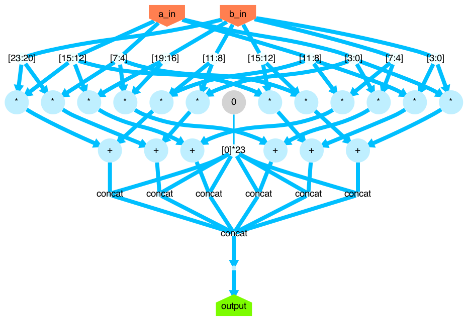
Synthesis Results
We’ve successfully created a RTL design that performs the same calculation as example_matrix_multiply.
Now, let’s synthesize it down to a netlist, and compare it with and without optimization.
Before doing so, thought, let’s write a function that gets some interesting information about the block.
def print_info(name):
    ta = pyrtl.TimingAnalysis()
    print(f"Max frequency: {ta.max_freq()} MhZ")
    print(f"Max timing delay: {ta.max_length()} ps")
    print(f"Logic count: {len({l for l in pyrtl.working_block().logic if l.op not in 'wcs'})}")
    logic, _ = pyrtl.area_estimation()
    print(f"Logic area est: {logic}")
    with open(f"{name}.v", 'w') as f:
        pyrtl.output_to_verilog(f)
    with open(f"{name}.gv", 'w') as f:
        pyrtl.output_to_graphviz(f)
To see if our intrinsic-based example_matrix_multiply is really better than standard matrix multiplication in terms of speed and resources, we’ll first create baseline hardware that uses PyRTL’s general-purpose matrix multiplication operator.
Here’s some code that does so [3]:
>>> a00, a01, a10, a11 = pyrtl.input_list('a00/4 a01/4 a10/4 a11/4')
>>> b00, b01, b02, b10, b11, b12 = pyrtl.input_list('b00/4 b01/4 b02/4 b10/4 b11/4 b12/4')
>>> a = Matrix.Matrix(2, 2, 4, value=[[a00, a01], [a10, a11]])
>>> b = Matrix.Matrix(2, 3, 4, value=[[b00, b01, b02], [b10, b11, b12]])
>>> output = Output(name='output')
>>> c = a @ b
>>> output <<= c.to_wirevector()
>>>
>>> sim = Simulation()
>>> sim.step({
>>>    'a00': a_vals[0][0], 'a01': a_vals[0][1], 'a10': a_vals[1][0], 'a11': a_vals[1][1],
>>>    'b00': b_vals[0][0], 'b01': b_vals[0][1], 'b02': b_vals[0][2],
>>>    'b10': b_vals[1][0], 'b11': b_vals[1][1], 'b12': b_vals[1][2]
>>> })
>>> raw_matrix = Matrix.matrix_wv_to_list(sim.inspect('output'), c.rows, c.columns, c.bits)
>>> raw_matrix
[[18, 24, 30], [38, 52, 66]]
We call pyrtl.synthesize() so that both designs are composed solely of primitive gates (like AND and OR) for an accurate comparison.
Then calling our helper print_info() on the baseline and our custom instrinsic-based design (both before and after calling pyrtl.optimize()) produces the results in the following table.
| Max Frequency (MhZ) | Max Timing Delay (ps) | Logic Count (non-wsc gates) |
Logic Area Estimate (mm^2) | |
|---|---|---|---|---|
Naive, pre-optimization |
270.88 |
3308.58 |
6288 |
0.0643 |
Custom, pre-optimization |
310.13 |
2841.44 |
1680 |
0.0186 |
Naive, post-optimization |
349.60 |
2477.39 |
1470 |
0.0163 |
Custom, post-optimization |
359.67 |
2397.27 |
1266 |
0.0141 |
Taking a look at the first two rows of these post-synthesis results, our pre-optimization instrinsic-based design has an estimated maximum frequency of 310 MhZ, while the standard version using PyRTL matrix mulitply has an estimated frequency of 270 MhZ. The standard PyRTL version has 3.74x more gates (6288/1680) and takes up 3.46x more area (0.064399104/0.018608832) than our specialized version, before optimization.
However, it’s probably more useful to compare them after calling pyrtl.optimize(), which is what those bottom two rows are doing.
Our post-optimization instrinsic-based design has an estimated maximum frequency of 349.60 MhZ, while the standard version has an estimated frequency of 359.67 MhZ.
The standard PyRTL version has 1.16x more gates (1470/1266) and takes up 1.15x more area.
After automatic optimization, our instrinsic-based design still does better than the standard PyRTL matrix multiply version, though the gap is much smaller in this case. PyRTL’s optimizer, which involves constant propagation and common subexpression elimination, is doing a pretty good job at nearly matching our hand-tuned, optimized version. Pretty cool!
Source
1. We could also just use
numpy.matmul. Also note that I’m passing in a list c to fill to be consistent with the C version.
2. I’m passing in wires, rather than constants (which is also acceptable) to the Matrix initializers so that when we later call PyRTL’s
optimize() function, constant propagation doesn’t just get rid of everything and so we can have a fair comparison.
3. I’m passing in values for the Matrices a little differently than previously, for the sole purpose of showing another way of doing it. They are equivalent, though there is an obvious tradeoff in verbosity vs. clarity of what’s going on.